Visual Predictive Checks (VPC)
Benjamin Guiastrennec
01 March, 2026
Source:vignettes/vpc.Rmd
vpc.RmdDisclosure
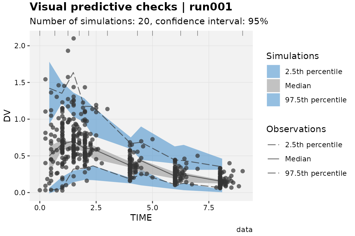
The Visual predictive checks (VPC) shown below are only intended to
demonstrate the various options available in xpose and should not be
used as reference for modeling practice. Furthermore, the plots are only
based on 20 simulations to minimize the computing time of the examples,
the size of the xpdb_ex_pk object and of the xpose package
in general.
Introduction
VPC can be created either by:
- Using an xpdb containing a simulation and an estimation problem
- Using a PsN generated VPC folder
The VPC functionality in xpose is build around the vpc R package. For more details about the way the vpc package works, please check the github repository.
Workflow
The VPC computing and plotting parts have been separated into two
distinct functions: vpc_data() and vpc()
respectively. This allows to:
- Optimize the speed when adjusting the graphics aesthetics
- Adjust the VPC data (e.g. remove panels or factor labels) before plotting
- Facilitate error debugging
The generated VPC data is stored in the xpdb under specials datasets and can be used later on.
xpdb_w_vpc <- vpc_data(xpdb_ex_pk) # Compute and store VPC data

xpdb_w_vpc # The vpc data is now listed under the xpdb "special" data
run001.lst overview:
- Software: nonmem 7.3.0
- Attached files (memory usage 1.5 Mb):
+ obs tabs: $prob no.1: catab001.csv, cotab001, patab001, sdtab001
+ sim tabs: $prob no.2: simtab001.zip
+ output files: run001.cor, run001.cov, run001.ext, run001.grd, run001.phi, run001.shk
+ special: vpc continuous (#3)
- gg_theme: theme_readable
- xp_theme: theme_xp_default
- Options: dir = data, quiet = FALSE, manual_import = NULL
vpc(xpdb_w_vpc) # Plot the vpc from the stored data
Multiple VPC data can be stored in an xpdb, but only one of each
vpc_type.
Common options
Options in vpc_data()
- The option
vpc_typeallows to specify the type of VPC to be computed: “continuous” (default), “categorical”, “censored”, “time-to-event”. - The
stratifyoptions defines up to two stratifying variable to be used when computing the VPC data. Thestratifyvariables can either be provided as a character vector (stratify = c('SEX', 'MED1')) or a formula (stratify = SEX~MED1) . The former will result in the use ofggforce::facet_wrap_paginate()and the latter ofggforce::facet_grid_paginate()when creating the plot. With “categorical” VPC the “group” variable will also be added by default. - More advanced options (i.e. binning, pi, ci, predcorr, lloq, etc.)
are accessible via the
optargument. Theoptargument expects the output from thevpc_opt()functions argument.
Options in vpc()
- The option
vpc_typeworks similarly tovpc_data()and is only required if several VPC data are associated with the xpdb. - The option
smooth = TRUE/FALSEallows to switch between smooth and squared shaded areas. - The plot VPC function works similarly to all other xpose functions
to map and customize aesthetics. However in this case the
area_fillandline_linetypeeach require three values for the low, median and high percentiles respectively.
Creating VPC using the xpdb data
To create VPC using the xpdb data, at least one simulation and one
estimation problem need to present. Hence in the case of NONMEM the run
used to generate the xpdb should contain several$PROBLEM.
In vpc_data() the problem number can be specified for the
observation (obs_problem) and the simulation
(sim_problem). By default xpose picks the last one of each
to generate the VPC.
# View the xpdb content and data problems
xpdb_ex_pk
run001.lst overview:
- Software: nonmem 7.3.0
- Attached files (memory usage 1.5 Mb):
+ obs tabs: $prob no.1: catab001.csv, cotab001, patab001, sdtab001
+ sim tabs: $prob no.2: simtab001.zip
+ output files: run001.cor, run001.cov, run001.ext, run001.grd, run001.phi, run001.shk
+ special: <none>
- gg_theme: theme_readable
- xp_theme: theme_xp_default
- Options: dir = data, quiet = FALSE, manual_import = NULL
# Generate the vpc
xpdb_ex_pk %>%
 vpc_data(vpc_type = 'continuous', obs_problem = 1, sim_problem = 2) %>%
 vpc()
Creating the VPC using a PsN folder
The vpc_data() contains an argument
psn_folder which can be used to point to a PsN generated VPC
folder. As in most xpose function template_titles keywords
can be used to automatize the process
e.g. psn_folder = '@dir/@run_vpc' where @dir
and @run will be automatically translated to initial
(i.e. when the xpdb was generated) run directory and run number
'analysis/models/pk/run001_vpc'.
In this case, the data will be read from the /m1
sub-folder (or m1.zip if compressed). Note that PsN drops unused
columns to reduce the simtab file size. Thus, in order to allow for more
flexibility in R, it is recommended to use multiple stratifying
variables (-stratify_on=VAR1,VAR2) and the prediction
corrected (-predcorr adds the PRED column to the output)
options in PsN to
avoid having to rerun PsN to add these
variables later on. In addition, -dv, -idv,
-lloq, -uloq, -predcorr and
-stratify_on PsN options are
automatically applied to xpose VPC.
The PsN generated binning can also applied to xpose VPC with the
vpc_data() option psn_bins = TRUE (disabled by
default). However PsN and the vpc
package work slightly differently so the results may not be optimal and
the output should be evaluated carefully.