Introduction
Benjamin Guiastrennec
01 March, 2026
Source:vignettes/introduction.Rmd
introduction.RmdImport model output
The function xpose_data() collects all model output
files and table and organizes them into an R object commonly called
xpdb which stands for “xpose database”.
xpdb <- xpose_data(runno = '001', dir = 'analysis/model/pk/')Glimpse at the xpdb
The files attached to an xpdb object can be displayed to the console
simply by writing its name to the console or by using the
print() function.
xpdb # or print(xpdb)run001.lst overview:
- Software: nonmem 7.3.0
- Attached files (memory usage 1.4 Mb):
+ obs tabs: $prob no.1: catab001.csv, cotab001, patab001, sdtab001
+ sim tabs: $prob no.2: simtab001.zip
+ output files: run001.cor, run001.cov, run001.ext, run001.grd, run001.phi, run001.shk
+ special: <none>
- gg_theme: theme_readable
- xp_theme: theme_xp_default
- Options: dir = data, quiet = FALSE, manual_import = NULLModel summary
A summary of a model run can be displayed to the console by using the
summary() function on an xpdb object.
summary(xpdb)
Summary for problem no. 0 [Global information]
 - Software                      @software   : nonmem
 - Software version              @version    : 7.3.0
 - Run directory                 @dir        : data
 - Run file                      @file       : run001.lst
 - Run number                    @run        : run001
 - Reference model               @ref        : 000
 - Run description               @descr      : NONMEM PK example for xpose
 - Run start time                @timestart  : Mon Oct 16 13:34:28 CEST 2017
 - Run stop time                 @timestop   : Mon Oct 16 13:34:35 CEST 2017

Summary for problem no. 1 [Parameter estimation]
 - Input data                    @data       : ../../mx19_2.csv
 - Number of individuals         @nind       : 74
 - Number of observations        @nobs       : 476
 - ADVAN                         @subroutine : 2
 - Estimation method             @method     : foce-i
 - Termination message           @term       : MINIMIZATION SUCCESSFUL
 - Estimation runtime            @runtime    : 00:00:02
 - Objective function value      @ofv        : -1403.905
 - Number of significant digits  @nsig       : 3.3
 - Covariance step runtime       @covtime    : 00:00:03
 - Condition number              @condn      : 21.5
 - Eta shrinkage                 @etashk     : 9.3 [1], 28.7 [2], 23.7 [3]
 - Epsilon shrinkage             @epsshk     : 14.9 [1]
 - Run warnings                  @warnings   : (WARNING 2) NM-TRAN INFERS THAT THE DATA ARE POPULATION.

Summary for problem no. 2 [Model simulations]
 - Input data                    @data       : ../../mx19_2.csv
 - Number of individuals         @nind       : 74
 - Number of observations        @nobs       : 476
 - Estimation method             @method     : sim
 - Number of simulations         @nsim       : 20
 - Simulation seed               @simseed    : 221287
 - Run warnings                  @warnings   : (WARNING 2) NM-TRAN INFERS THAT THE DATA ARE POPULATION.
                                               (WARNING 22) WITH $MSFI AND "SUBPROBS", "TRUE=FINAL" ...
Parameter estimates
A table of parameter estimates can be displayed to the console by
using the prm_table() function on an xpdb object.
prm_table(xpdb)
Reporting transformed parameters:
For the OMEGA and SIGMA matrices, values are reported as standard deviations for the diagonal elements and as correlations for the off-diagonal elements. The relative standard errors (RSE) for OMEGA and SIGMA are reported on the approximate standard deviation scale (SE/variance estimate)/2. Use `transform = FALSE` to report untransformed parameters.

Estimates for $prob no.1, subprob no.1, method foce
 Parameter  Label      Value        RSE
 THETA1     TVCL       26.29        0.03391
 THETA2     TVV        1.348        0.0325
 THETA3     TVKA       4.204        0.1925
 THETA4     LAG        0.208        0.07554
 THETA5     Prop. Err  0.2046       0.1097
 THETA6     Add. Err   0.01055      0.3466
 THETA7     CRCL on CL 0.007172     0.2366
 OMEGA(1,1) IIV CL     0.2701       0.08616
 OMEGA(2,2) IIV V      0.195        0.1643
 OMEGA(3,3) IIV KA     1.381        0.1463
 SIGMA(1,1)            1        fix  -
Listing variables
A list of available variables for plotting can be displayed to the
console by using the list_vars() function on an xpdb
object.
list_vars(xpdb)
List of available variables for problem no. 1
 - Subject identifier (id)               : ID
 - Dependent variable (dv)               : DV
 - Independent variable (idv)            : TIME
 - Dose amount (amt)                     : AMT
 - Event identifier (evid)               : EVID
 - Model typical predictions (pred)      : PRED
 - Model individual predictions (ipred)  : IPRED
 - Model parameter (param)               : KA, CL, V, ALAG1
 - Eta (eta)                             : ETA1, ETA2, ETA3
 - Residuals (res)                       : CWRES, IWRES, RES, WRES
 - Categorical covariates (catcov)       : SEX, MED1, MED2
 - Continuous covariates (contcov)       : CLCR, AGE, WT
 - Compartment amounts (a)               : A1, A2
 - Not attributed (na)                   : DOSE, SS, II, TAD, CPRED

List of available variables for problem no. 2
 - Subject identifier (id)               : ID
 - Dependent variable (dv)               : DV
 - Independent variable (idv)            : TIME
 - Dose amount (amt)                     : AMT
 - Event identifier (evid)               : EVID
 - Model individual predictions (ipred)  : IPRED
 - Not attributed (na)                   : DOSE, TAD, SEX, CLCR, AGE, WT
Pipes
xpose makes use of the pipe operator %>%
from the package dplyr. Pipes
can be used to generate clear workflow.
xpose_data(runno = '001') %>%
  dv_vs_ipred() %>%
  xpose_save(file = 'run001_dv_vs_ipred.pdf')
Editing the xpdb
Multiples edits can be made to the xpdb object. For instance the type
(visible using the list_vars() function described above) of
a variable can be changed. Hence the independent variable (idv) could be
changed from TIME (default in NONMEM) to TAD.
All plots using idv will then automatically use
TAD.
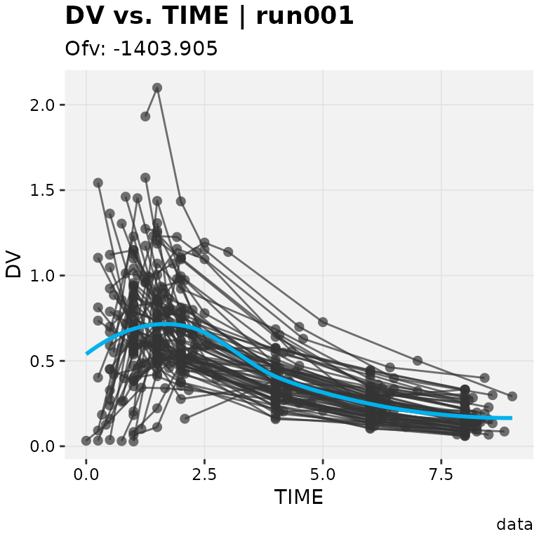
# After IDV reassignment
xpdb %>%
  set_var_types(idv = 'TAD') %>%
  dv_vs_idv()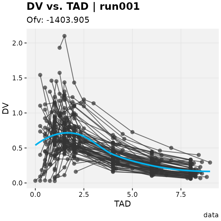
Generating plots
Plotting functions are used as follows:
# DV vs. IPRED plot
dv_vs_ipred(xpdb)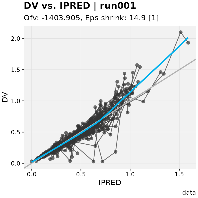
# CWRES vs. PRED plot
res_vs_pred(xpdb, res = 'CWRES')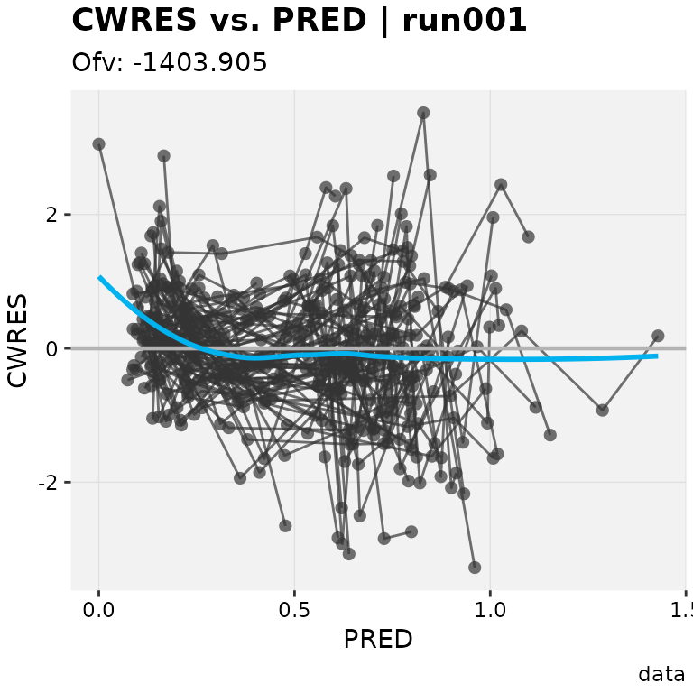
Saving plots
The xpose_save function was designed to facilitate the
export of xpose plots. The file extension is guessed from the file name
and must match one of .pdf (default), .jpeg, .png, .bmp or .tiff. If no
extension is provided as part of the file name a .pdf will be generated.
Finally, if the plot argument is left empty
xpose_save will automatically save the last plot that was
created or modified.
The xpose_save() function is compatible with templates
titles and keywords such as @run for the run number and
@plotfun for the name of the plotting function can be used
to automatically name files. Learn more about the template titles
keywords using help('template_titles').
# Save the last generated plot
dv_vs_ipred(xpdb)
xpose_save(file = 'run001_dv_vs_ipred.pdf')

# Template titles can also be used in filename and the directory
xpdb %>%
 dv_vs_ipred() %>%
 xpose_save(file = '@run_@plotfun_[@ofv].jpeg', dir = '@dir')